Uncertainty Quantification in Neural Mass Conserving Data Assimilation

Overview

The core problem the original paper solves is: improve data assimilation in a physically constrained shallow water model, by replacing an expensive (but accurate) heuristic approach with a neural approach. This on its own is a multi-stage research problem involving simulation, observation generation, classical assimilation baselines and learning correction models.

This repository puts these pieces together into one end-to-end workflow and expands on top of it with an Uncertainty quantification pipeline using Conformal Prediction (CP) and Conformalized Quantile Regression (CQR).

End-to-end pipeline

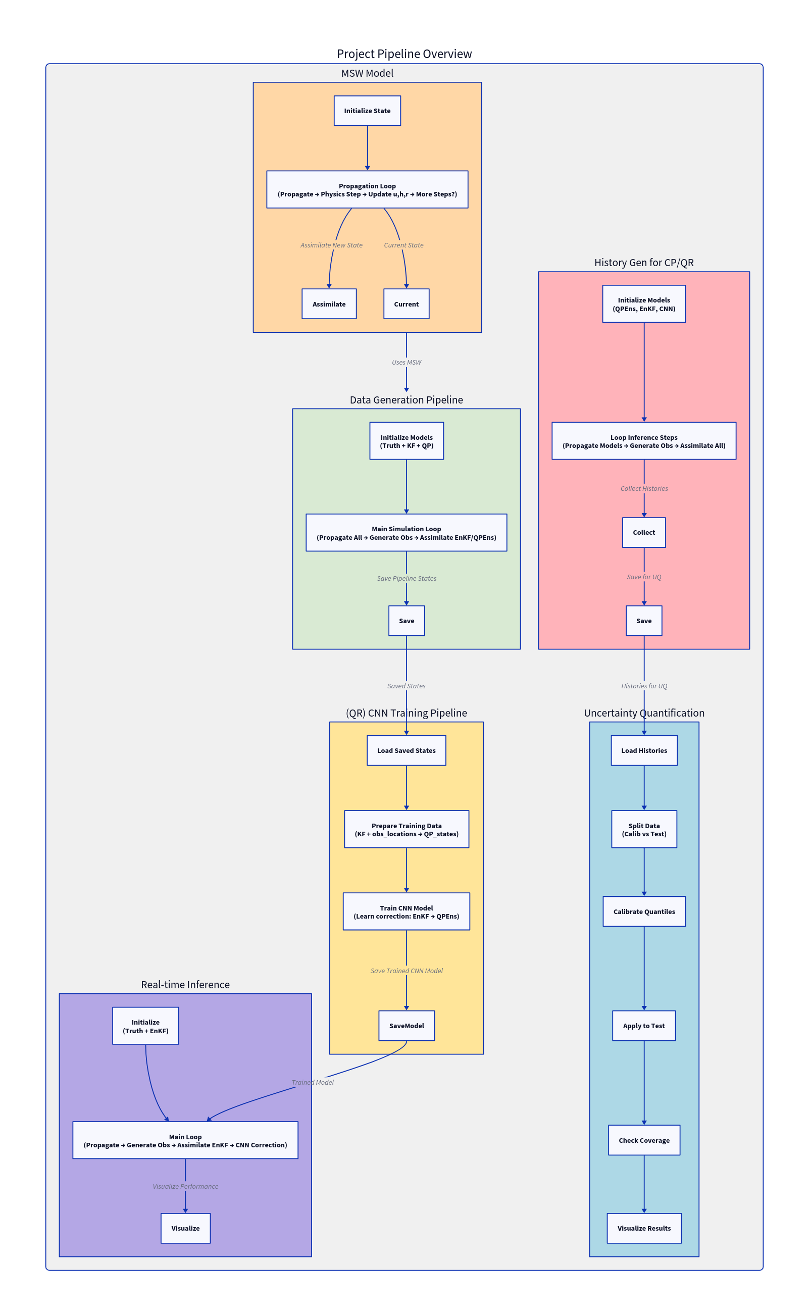
1. Physical model backbone

The whole system begins with the MSW model, which provides the controlled physical environment. A single MSW state tracks variables such as velocity, water height, and rain over a spatial grid and evolves them under shallow-water dynamics with stochastic perturbations.

This physical constraints are required because the later ML components are only meaningful if the upstream dynamics are physically grounded.

2. Training-data generation for data assimilation

Once the physical simulator is set up, the next step is to generate training data that makes the correction problem learnable. Therefore a ground truth model is propagated, from which noisy and masked observations are constructed. In addition, separately EnKF and QPEns model states are propagated. The goal is to use the noisy generated obsevations stemming from the ground truth model, to update the Ensemble Kalman Filter (EnKF) and Quadratic Programming Ensemble QPEns states to be as close as possible to the current ground truth state. The QPEns appraoch solves a constrained optimization problem given a set of constraints to calculate the optimal update given the observations (implementation details can be found here: https://github.com/OlegTolochko/msw-da-ml/blob/master/msw_da_ml/msw/assimilation.py)

This stage is especially important because it defines the training signal for the CNN. The CNN training objective is to map the more accessible EnKF behavior toward the stronger (but significantly more computationally expensive) QPEns target correction. This also involves an important design choice: Before assimilation in the EnKF model, the EnKF model state is set to previous QPEns model state. Since the pipeline is only used for training data generation and the target for the CNN is the QPEns prediction, the previous state input should also be a QPEns prediction. This is essentially equivalent to teacher forcing in seq2seq models.

This creates a set of pairs where X = EnKF correction and Y = QPEns correction.

3. CNN and quantile-regression training

To train the model a dataset is constructed from all generated EnKF and QPEns assimilation state pairs. The is trained to refine EnKF updates to match QPEns updates. (Side Note: The CNN also receives the observation locations as an additional input, besides the EnKF correction) EnKF updates on their own already relatively good and cheap to compute (This resembles the idea of anchors in object detection models in spirit). So the model is not required to directly perform the whole update. This turns the complex system-imitation problem to a simplified refinement problem.

So put simply: The CNN receives the not perfect EnKF update and refines it to be closer to the QPEns update, so essentially EnKF + CNN is supposed to be a cheaper alternative to QPEns.

The repository also includes a quantile-regression variant, which makes it possible to learn interval predictions (so upper and lower bound for each output variable) that later plug naturally into the uncertainty-quantification stage.

4. Inference loop

At inference time, the system returns to the original dynamical setting: propagate the ensemble, generate observations, assimilate with EnKF, and then apply the learned correction model. Optionally, QPEns can still be computed as a reference for comparison.

The main inference pipeline is a loop that can be run over many inference steps and evaluated operationally against truth and baseline methods.

5. History generation for evaluation

To evaluate uncertainty methods properly, the repository generates multi-seed histories across truth, EnKF, QPEns, and CNN-based predictions.

6. Uncertainty quantification

The main new research addition is an uncertainty quantification pipeline built on top. Two main routes are implemented:

• Conformal Prediction (CP), where non-conformity scores are calibrated and then converted into intervals on held-out data.
• Conformalized Quantile Regression (CQR), where learned lower and upper quantiles are widened just enough to achieve empirical coverage.

Also additional baselines such as MCDO, NIG-based evidential regression, normalized CP, and random-forest-style variants are included.

CLI

The repository is organized around a clean CLI surface in msw_da_ml.main. The main steps are:

uv sync

uv run python -m msw_da_ml.main generate-training-data
uv run python -m msw_da_ml.main train-cnn-model <training_data_name>
uv run python -m msw_da_ml.main train-quantile-regression-model <generated_msw_data_name>
uv run python -m msw_da_ml.main run-inference
uv run python -m msw_da_ml.main generate-conformal-prediction-data
uv run python -m msw_da_ml.main generate-cqr-data
uv run python -m msw_da_ml.main compare-uq-methods <cp_hist_name> <cqr_hist_name>